Like many, I have been fascinated by the Rubik’s cube since its introduction in 1979.
In 2011, I decided to leverage some of the image processing capabilities in Mathematica to solve the cube from 2 pictures. Here is what this will cover. (I gave this talk at the conference in October)
First let me summarize the key steps:
Quick Overview
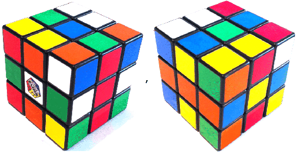
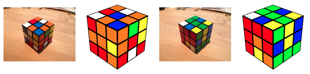
Input 2 pictures (taken by phone)
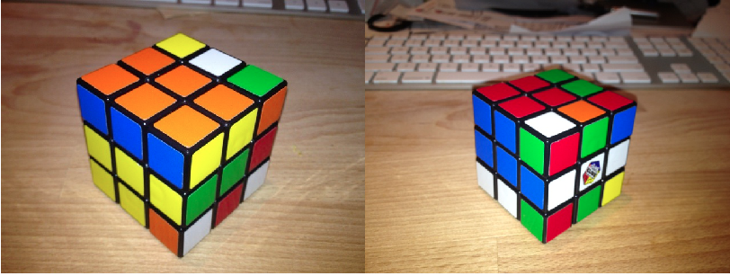
Then we do some image processing with Mathematica:

Then we rotate the cube to a canonical representation preferred by the solver
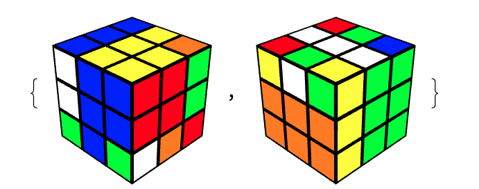

Then solve using a TwoPhase solver written in Mathematica (Special thanks to Herbert Kociemba for the two phase algorithm…)
< wlcode >solveCube c={{{7,2,1,6,8,3,4,5},{1,2,1,0,0,1,2,2}},{{2,10,4,6,7,11,8,12,9,5,3,1},{0,0,0,0,1,0,0,0,0,1,0,0}}}
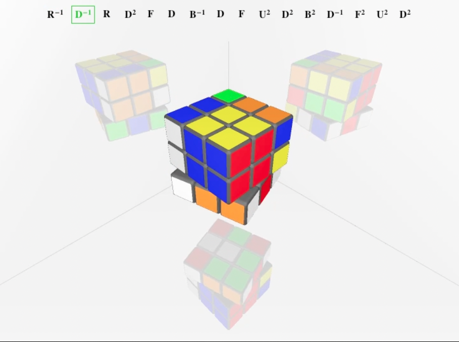
Then, output a movie using Mathematica
Let’s talk a bit about the process to get this to work:
The image processing solution is an optimization => collection of pictures to get a good sample
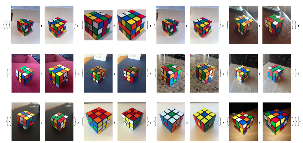
I got as many pictures as possible of cubes…
Then I started experiments in image processing:
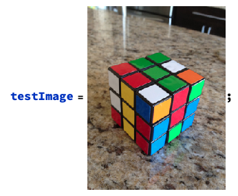
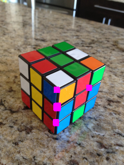
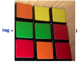
A sample image:
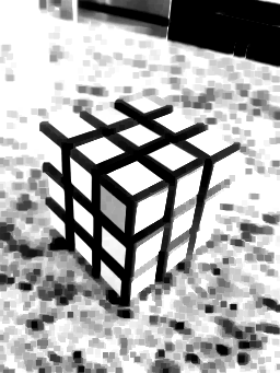
Color reduction:
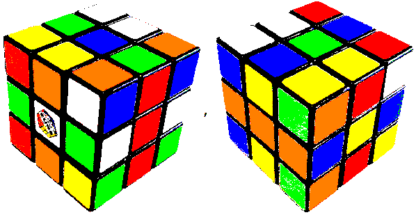
Erosion:
Edge Detection:
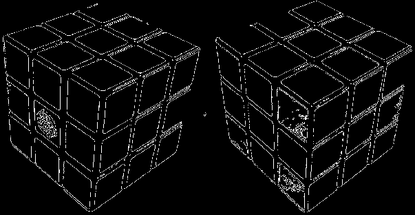
Image Lines:
Actual Implementation:
< wlcode >makeGrey256[img_] := Module[{step1},
step1 = ImageApply[Max[#] &, ImageResize[ImageAdjust[img, {.25, 0}], 256]];
ImageFilter[Min, ImageAdjust[step1,
Quantile[Flatten[ImageData[step1]], {0.05, .95}], {0, 1}], 2]];
greyImage = makeGrey256[testImage]
ImageCorrelate, MorphologicalComponents, ComponentMeasurements

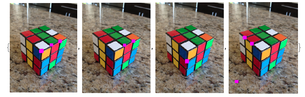
< wlcode >ImageApply[{1, 0, 1} &, ImageResize[testImage, 256],
Masking ->Dilation[ImageApply[1 – # &,
Binarize[ImageAdjust[ImageCorrelate[ greyImage, #,
NormalizedSquaredEuclideanDistance]], .05]], 5]
] & /@ kernelsForCenter
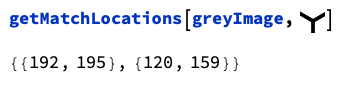
getMatchLocations[img_, kernel_] := Module[{matchPointImage, components, level = 0.022},(0.022)
matchPointImage = ColorNegate[ Binarize[ ImageAdjust[
ImageCorrelate[img, kernel, NormalizedSquaredEuclideanDistance]], level]];
components = MorphologicalComponents[matchPointImage];
Round[Last[#]] & /@ ComponentMeasurements[components, “Centroid”]];
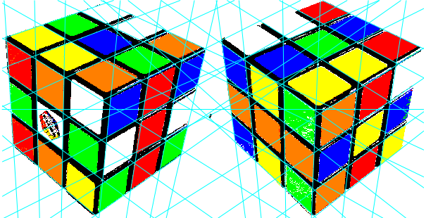
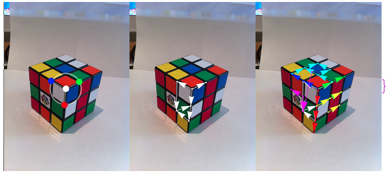
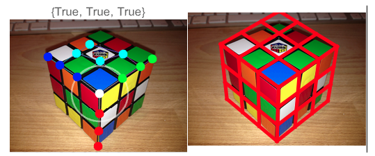
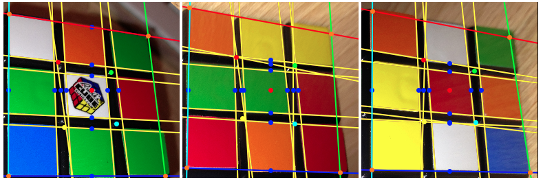
Add some graphs: DelaunayTriangulation, then select and orient the edges.
For example:
Solve the projection Matrix (using Solve to find rotations and FindMinimum to find the Cube distance and Focal Length)
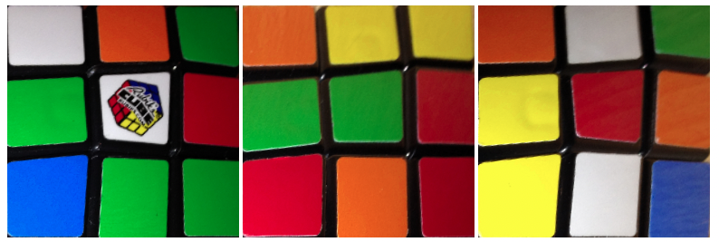
Use simple texture mapping to extract and renormalize the side views
< wlcode >Graphics[{Texture[img],Polygon[Map[Reverse,Flatten[Table[{{x, y}, {x, y + 1}, {x + 1, y + 1}, {x + 1, y}}, {x, 0,2}, {y, 0, 2}], 1], {2}],VertexTextureCoordinates -> Map[(origin + pjct[mat . #])/resizedDimentions &,
Flatten[Table[{{x, y, 0, 1}, {x, y + 1, 0, 1}, {x + 1, y + 1, 0,
1}, {x + 1, y, 0, 1}}, {x, 0, 2}, {y, 0, 2}], 1], {2}]]},
PlotRangePadding -> None, ImagePadding -> None, AspectRatio -> 1,
ImageSize -> {256, 256}]
Use GradientFilter and ImageLines to optimize the side views
< wlcode >makeGrey256[img_] :=Module[{step1},step1 = ImageApply[Max[#] &, ImageResize[ImageAdjust[img, {.25, 0}], 256]];
ImageFilter[Min,ImageAdjust[step1, Quantile[Flatten[ImageData[step1]], {0.05, .95}], {0, 1}], 2]];
< wlcode >temp = DeleteSmallComponents[
Binarize[ImageAdjust[ImageAdd[GradientFilter[makeGrey256[img], 1],
GradientFilter[img, 1]]]], 100]
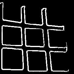
Get the ImageLines:
Apply texture mapping again
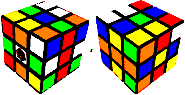
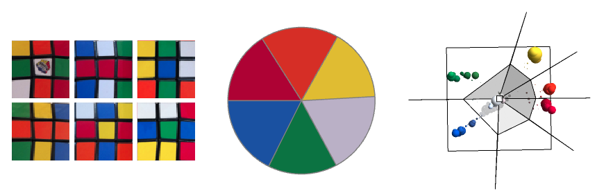
Apply magical color reduction…
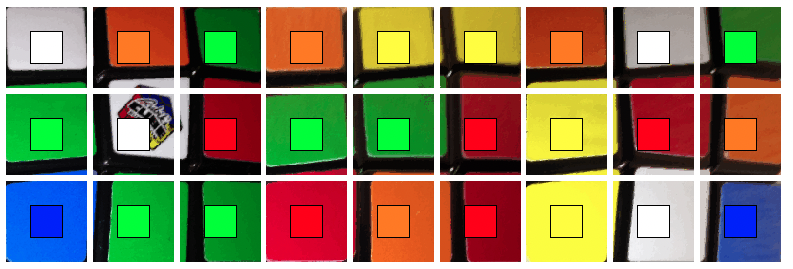
Image Processing – Color
Typical Problem in color space:
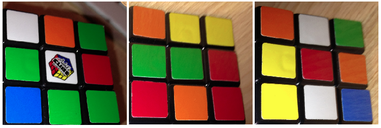
Because of lighting, color identification is quite a difficult problem:
Here are some examples:
Color space visualization:
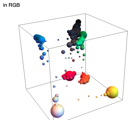
In HSB:
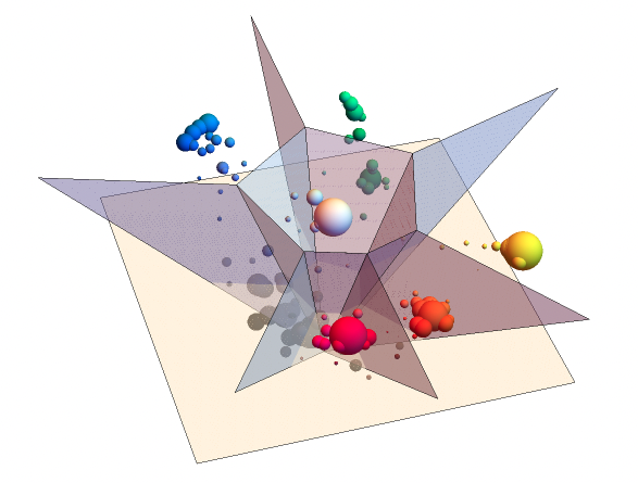
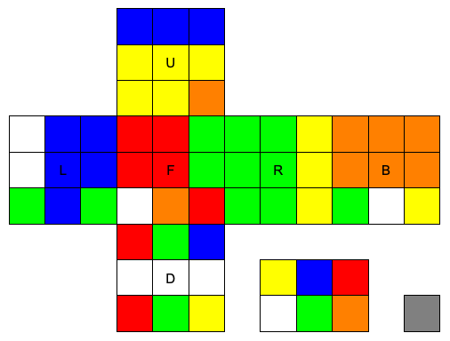
Solution is to extract all 6 faces, and then adjust the color matching
The two phase algorithm (written by Herbert Kociemba)
all details are at http://kociemba.org/cube.htm
Group of cubic moves is divided by G1 generated by U,D,R2,L2,F2,B2
Requires the Cube to be rotated in special position (Cube permutations to rotate in position)
Solver returns a series of moves
< wlcode >{“U1 “, “U2 “, “U3 “, “R1 “, “R2 “, “R3 “, “F1 “, “F2 “, “F3 “, “D1 \
“, “D2 “, “D3 “, “L1 “, “L2 “, “L3 “, “B1 “, “B2 “, “B3 “}
Build Movie from the solution
Cube rendering and animation
rendered as a series of move then transform…
The cube itself
mini cubes are ContourPlot3D
Label on faces are a single polygon
Cube itself is rendered by GeometricTransformation and Rotations
Example: a rotation of the front face
Table[GeometricTransformation[{
(* the labels on the cube *)
< wlcode >Table[{If[x == -1, {ColorList[[3z – y + 41]], GeometricTransformation[$aFace, {RotationMatrix[ Pi/2, {0, 1, 0}], {-1.5, y, z}}]}, {}], If[x == 1, {ColorList[[3z + y + 14]],
GeometricTransformation[$aFace, {RotationMatrix[Pi/2, {0, 1, 0}], {1.5,y, z}}]}, {}],
If[y == -1, {ColorList[[3z + x + 32]], GeometricTransformation[$aFace, {RotationMatrix[ Pi/2, {1, 0, 0}], {x, -1.5, z}}]}, {}], If[y == 1, {ColorList[[3z – x + 23]],
GeometricTransformation[$aFace, {RotationMatrix[Pi/2, {1, 0, 0}], {x,1.5, z}}]}, {}],
If[z == -1, {ColorList[[-3y + x + 50]], GeometricTransformation[$aFace, {IdentityMatrix[3], {x, y, -1.5}}]}, {}], If[z == 1, {ColorList[[3y + x + 5]],
GeometricTransformation[$aFace, {IdentityMatrix[3], {x, y,1.5}}]}, {}]}, {y, -1, 1}, {z, -1, 1}],
(* the mini cubes themselves *)
< wlcode >GeometricTransformation[{cube3DObject[[1]]},
Flatten[Table[{IdentityMatrix[3], {x, y, z}}, {y, -1, 1}, {z, -1, 1}],
1]]}, {{IdentityMatrix[3]}, {IdentityMatrix[
3]}, {RotationMatrix[-angle, {1, 0, 0}]}}[[{x + 2}]]]
, {x, -1, 1}],
The Scene
The scene itself is a series of GeometricTransformation
< wlcode >GeometricTransformation[
…
{{IdentityMatrix[3], {0, 0, 0}},
{ReflectionMatrix[{1, 0, 0}], {-7, 0, 0}},
{ReflectionMatrix[{0, 1, 0}], {0, 7, 0}},
{ReflectionMatrix[{0, 0, 1}], {0, 0, -7}}
}
]
The reflections are seen through low transparency polygons, which give the illusion of reflection
Polygon[{center, center + {maxAxes, 0, 0}, center + {maxAxes, 0, maxAxes},
center + {0, 0, maxAxes}}], Polygon[{center, center + {maxAxes, 0, 0},
center + {maxAxes, -maxAxes, 0},
center + {0, -maxAxes, 0}}], Polygon[{center, center + {0, -maxAxes, 0},
center + {0, -maxAxes, maxAxes}, center + {0, 0, maxAxes}}],
The moves as Text are added as an Epilog.